Performance engineering in agentic AI systems

Enterprise AI has evolved from single-model Q&A toward orchestrated multi-agent systems. Businesses increasingly need AI that can reason across processes, understand internal documents and automate end-to-end operations. Naive designs scale poorly in predictable ways. Latency accumulates when independent steps run sequentially. Token costs grow with traffic instead of value. Reliability degrades when unstructured outputs break downstream parsers. And routing hallucinations invoke the wrong specialist, which is often costlier than a wrong final answer.

This article documents some optimizations that take a system from functional prototype to production-grade infrastructure, with real trade-off analysis at each step.

Before optimizing any workflow, measure it. Teams often spend weeks tuning prompts or introducing caching only to discover that the real bottleneck is a slow database call or an external API. Latency, token consumption and failure rates should be observable at every node in the graph before optimization begins.

Right-sizing models for agent workflows

The first and most impactful change is deceptively simple: stop using your best model for everything. An agentic workflow is a pipeline of small decisions and large syntheses. Treating every step as "call the frontier model" works in demos. At enterprise scale, it becomes an expensive and slow default.

The fix is to identify the distinct use-cases in the workflow and map the right model to each one explicitly. Even the same base model running at different temperatures or token limits should be treated as a different configuration, since these parameters change output behavior and cost. Evaluate candidate models and their parameters against each task type to find the right assignment, then externalise that mapping from the codebase entirely so it can be fetched at inference time. Changing a model assignment or tuning a parameter requires no code change, and the entire cost-quality trade-off across the system lives in one place.

A practical way to think about model assignment is by matching task complexity to model capability.

Prompt and API response caching

In enterprise settings, users frequently ask the same questions with minor variations in phrasing: "show me revenue by region last month," "regional breakdown for the past 30 days," "last month's revenue per region." Running the entire workflow afresh on every one of these is a wasted cost. Not every step needs to be re-run. 

What should be cached?

Steps like guardrail checks and intent classification produce the same result for semantically identical queries and can be short-circuited entirely. Steps like structured query generation can be cached with placeholders for the dynamic parts like date ranges and user IDs, and a small model fills those slots at query time rather than regenerating the full query from scratch. Steps like summarising freshly fetched data genuinely need to run each time, and they should. The goal is not to cache everything but to avoid re-running what does not need to change.

There are two distinct caching strategies at play here and they solve different problems. 

Key-value caching

Key-value caching works on exact or near-exact matches, which is the same query string hitting the same cached response. This handles strict repetition well but breaks down the moment a user rephrases the question even slightly. 

Semantic caching

Semantic caching addresses this by operating on meaning rather than string matching. The query is embedded and compared against cached responses in vector space. Instead of looking for an exact match, retrieve the top-k semantically similar responses and use a lightweight model to select the best candidate. This shifts what would have been a full generation task into a selection task, which is significantly cheaper and faster.

Async parallelization in agent graphs

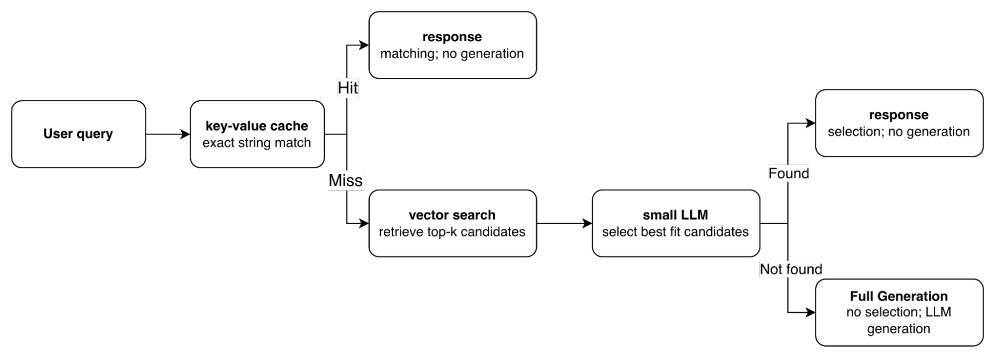
An agentic workflow may require multiple steps to address a single user request. Take a data analytics query as an example.

Analytics request:

→ Intent classification

→ Query generation

→ Data fetch

→ Code generation

→ Explanation generation

→ Follow-up suggestions

Each step can invoke an LLM, make an HTTP call or run deterministic processing.

In this example flow, the four steps after query generation (data fetch, code generation, explanation and follow-up suggestions) have no dependency on each other. They only depend on the query generated in the step before them. Yet the naive implementation runs them sequentially. If each step takes roughly three seconds, those four steps alone accumulate to about 12 seconds of wall-clock time, even though the true dependency graph would allow all four to run simultaneously.

The solution is a fan-out/fan-in pattern with query generation as the shared prerequisite. Once the query is ready, all four independent steps are dispatched concurrently and their results are merged at a barrier before the final response is assembled. User-visible latency shifts from the sum of the four branches to the maximum of them: roughly 3 seconds instead of 12 in this example.

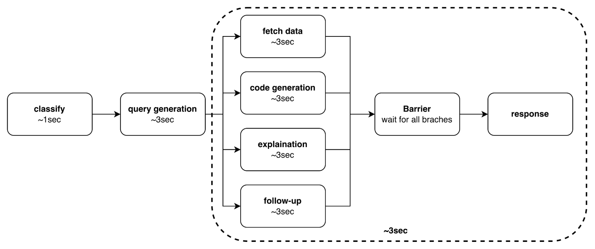
Three things need to be in place for this to work reliably:

• Where possible, artificial dependencies between steps should be removed. A downstream step that only needs the schema of the data, not the live values, can start before the data fetch completes.

• Concurrent branches writing to shared state need explicit merge rules (additive merges for lists, last-write-wins for scalars), otherwise race conditions surface silently under load.

• Each branch needs its own failure handling so a single branch error does not collapse the entire response.

Parallelization also opens up a useful distinction between hot and cold paths. (Not every step in a workflow needs to be completed before the user sees a response.) The hot path is the minimal set of steps required to deliver the primary answer. In the analytics example, that is query generation, data fetch and rendering the result. 

The cold path covers steps whose output enriches the experience but is not blocking: follow-up suggestions, logging, updating recommendation models or pre-warming caches for likely next queries. Cold path work can be dispatched asynchronously after the hot path response is returned, running in the background without contributing to user-visible latency. Identifying this split early in the workflow design often yields more latency reduction than parallelizing within the hot path alone.

When not to use fan-out

Do not parallelize when steps have genuine sequential dependencies, when per-branch observability is not in place or when partial-failure policies are not defined. Without a partial-failure policy, a branch that fails will pass incomplete state through the barrier silently, producing a broken response with no clear cause.

Partial deterministic flows and structured outputs

Even after removing unnecessary latency, another optimization opportunity remains: reducing the number of LLM calls altogether. Not everything in an agentic workflow needs an LLM. Many steps only appear to need one because the workflow was built that way by default. The principle is to use LLMs for the parts that genuinely require language understanding or reasoning, and handle everything else in code. Four patterns show where this split consistently pays off.

1. Query modification 

When an LLM generates a structured query and a filter needs to be added to it, the instinct is to ask the LLM to include it. But most structured query languages expose a parser: the filter can be injected by parsing the output and appending the clause in code, which is guaranteed to be placed correctly every time. 

2. Query reuse

Similarly, when a flow needs two queries with the same filters (one returning a count for user confirmation, another returning the actual entities), the second query does not need a fresh LLM call. The count query can be modified programmatically by swapping what is selected while keeping the filter conditions unchanged.

3. Tool-response transformation

In tool-chaining flows where one tool's response feeds into the next, the LLM does not need to see the full data payload to decide what to pass forward. If the response schema is known, the required fields can be extracted in code and injected into the second tool call directly, keeping large data payloads out of the context entirely. 

4. Schema-driven sample generation

When a parallel branch needs representative data to work with (such as the code generation step), if the schema is known, sample data can be generated programmatically. No LLM call, no risk of a hallucinated field name.

What ties all of these together is structured outputs. When LLM outputs are validated against a schema before being passed downstream, deterministic code can operate on them safely. Without schema validation, the boundary between LLM and code becomes fragile: a slightly malformed field or an unexpected key breaks the downstream step in ways that are hard to trace. With it, the contract between LLM and code is explicit, and the deterministic parts of the flow can be tested independently of the model.

Context engineering: Send less, get better results

There’s a tempting default in agentic AI systems: when in doubt, include more context. Give the model the full conversation history, all available user metadata, every relevant tool description and all retrieved documents. 

Sending everything as context, however, creates three compounding costs:

• More context increases latency because the model must process additional tokens before generating a response.

• Larger prompts increase cost directly.

• Irrelevant context dilutes signal and can reduce answer quality.

The fix is to treat context as a dynamic selection problem rather than a static inclusion problem. Prompt templates should be structured with typed slots: a slot for relevant tool definitions, a slot for retrieved documents, a slot for conversation turns and a slot for user-specific metadata. At request time, a context selection layer evaluates the user query and populates only the slots that are relevant to it. A question about data analytics does not need the HR policy tool definitions. A greeting does not need the last ten conversation turns. A routine lookup does not need the full user profile.

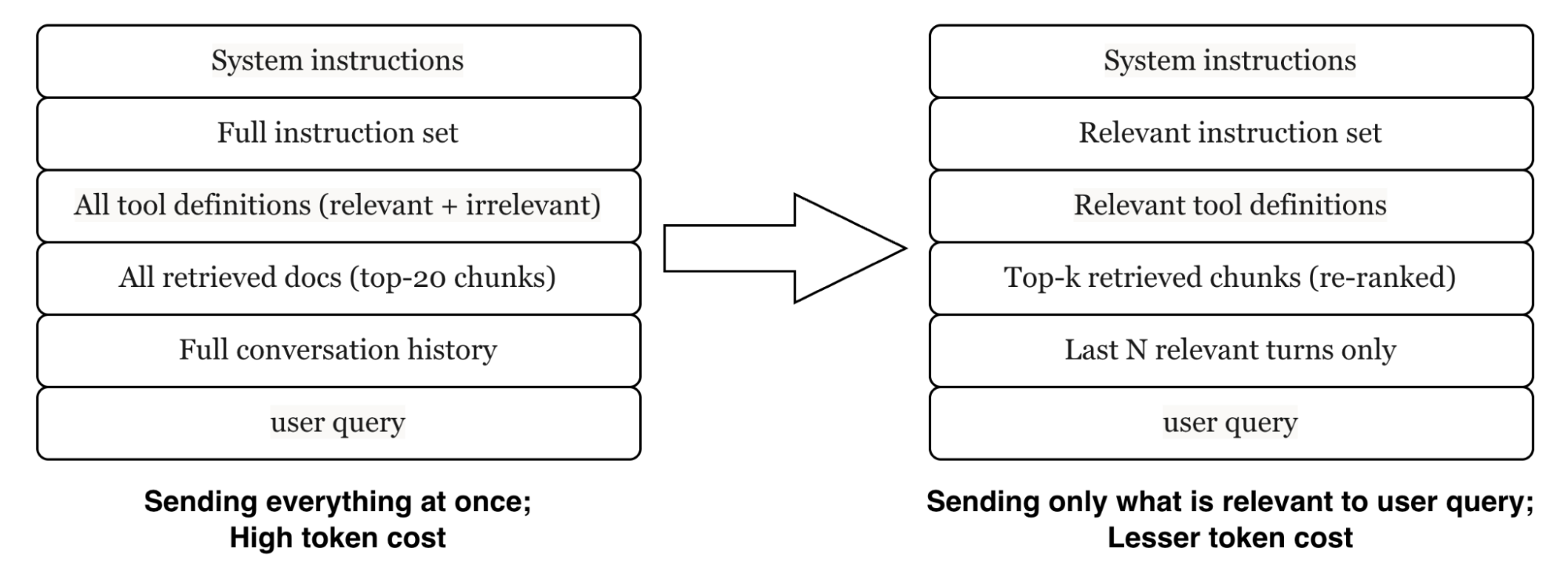
Implementing this requires a templated prompt structure where each context section is a named, optional slot, and a lightweight routing step that decides which slots to fill before the main LLM call. That routing step is cheap. It can be a similarity lookup against a slot-to-content index, a rule based on the classified intent or a small model call. The investment pays back on every subsequent LLM call in the graph, which sees a cleaner, shorter and more focused prompt.

What this may look like in practice

Define your prompt as a template with named sections: {{system}}, {{tools}}, {{retrieved_context}}, {{history}}, {{user_message}}. At request time, populate only the sections the query actually needs. Empty slots are omitted entirely, not filled with placeholder text.

Prompt structure and KV cache utilization

Once you've reduced the amount of context, the next optimization is arranging it to maximize prompt cache hits. The two concerns are complementary: get the content right first, then arrange it to maximize cache hits.

Most LLM providers maintain a key-value cache of attention computations across requests. When the prefix of a prompt matches a previously processed sequence exactly, the provider skips recomputing attention for that prefix and charges reduced or zero input tokens for the cached portion. This is a free latency and cost win, but only if you structure your prompts to exploit it.

The rule is straightforward: everything stable goes at the top, everything dynamic goes at the bottom. System instructions, tool definitions and fixed few-shot examples form a long, invariant prefix. The dynamically selected context and the user message slot in at the very end. When the next request arrives, the provider finds the cached prefix, skips it and only processes the short dynamic tail.

The connection to  context engineering is direct: dynamic context selection produces a shorter, cleaner dynamic tail, which means the cached prefix covers a larger fraction of the total prompt. The two optimizations compound. A statically ordered, fat prompt with everything included gets zero cache benefit on the dynamic portion and pays full token cost. A dynamically selected, ordered prompt gets the cache hit on the stable prefix and pays only for a small, focused tail.

One practical constraint: the moment you shuffle the order of any static block between requests, the prefix no longer matches and you forfeit the cache hit entirely. This means few-shot examples must be fixed and front-loaded, not dynamically reordered per query. If you need query-adaptive examples, place them in the dynamic section after the static prefix rather than mixing them into the static block. Most providers also require an explicit opt-in flag (Anthropic's cache_control breakpoint, OpenAI's prompt caching on supported models). Check that it’s active in your LLM gateway config before assuming the cache is doing anything.

Combined rule

First: select only what the query needs ( full context). Then: order the prompt as system → tools → fixed examples → selected context → user message. The static prefix gets cached. The dynamic tail stays small. Both savings stack.

Semantic similarity vs. LLM classification

Intent classification and routing are everywhere in agentic systems. For stable label spaces, semantic similarity often outperforms LLM-based classification on both cost and latency.

The main cost of adopting this approach is curating the initial example set. You need a representative labeled dataset for each class before the classifier is useful. This is the real trade-off: the LLM approach has near-zero setup cost (write a prompt, ship it) but high per-call cost and opaque failure modes. The similarity approach has an upfront curation cost but near-zero per-call cost and transparent failure modes (you can always inspect which examples are pulled in the wrong direction).

The better framing is to treat example curation as a pipeline, not a one-time task. Start with a manually curated seed set. Route low-confidence cases to an LLM, log the confirmed outcomes and add them back to the example store. Over time, fallback rates decline and classification quality improves.

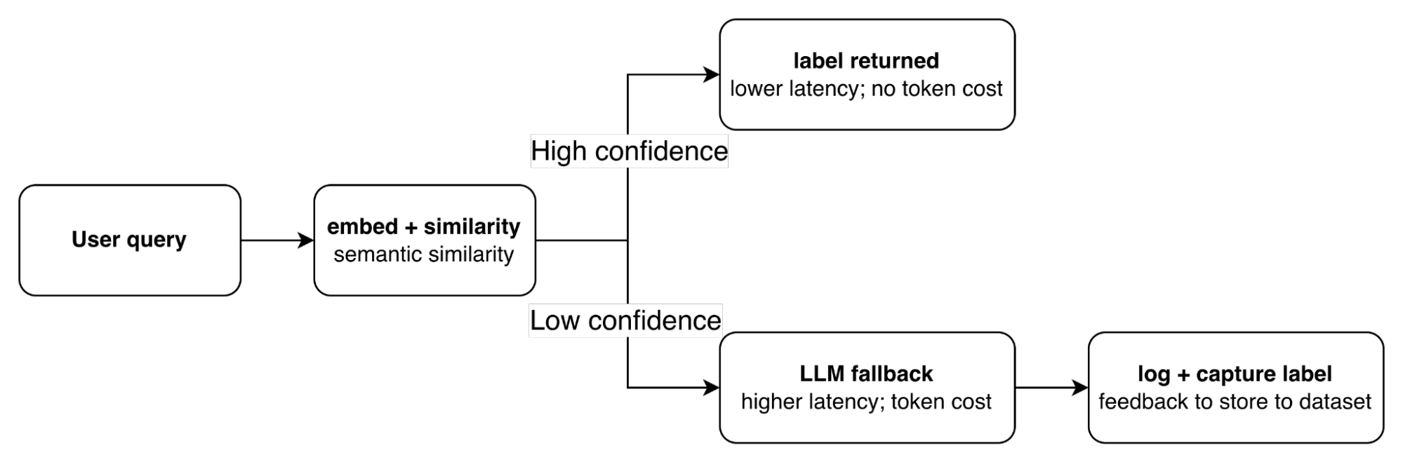
A practical threshold to start with is a cosine similarity score above 0.85 for a high-confidence accept, and below this for a hard LLM fallback. These numbers shift with your embedding model, label space and domain, but the structure holds. The classifier gets better with use rather than degrading as label drift accumulates in a static prompt.

The durable design tension

Every unnecessary LLM call becomes a cost, latency and reliability tax at scale. The techniques in this article all serve the same goal: reducing that tax through better routing, smarter orchestration and more deterministic execution.

The durable tension is four-way: flexibility, determinism, latency and cost. Platforms that optimize one dimension while ignoring others routinely re-platform under incident load. The teams that sustain production load treat agent graphs as distributed systems — with barriers, backpressure, failure domains and observability — rather than as prompt demos with extra steps. 

Visibility and control, not autonomous novelty, is what makes agentic AI systems operable at enterprise scale.