Enable javascript in your browser for better experience. Need to know to enable it? Go here.
Blogs Banner

Predicting star formation properties with deep learning

There are about 51 galaxies in the Milky Way’s Local Group, about 100,000 in our Local Supercluster, and 100 billion in all of the observable universe. Many of what we see as tiny specs are, in fact, galaxies, containing stars, which, in turn, may have their own solar systems, planets and satellites. While these galaxies may seem inactive in our lifetime, many activities occur at a macro timescale — stars are born, they collapse, merge; there’s dust in the galaxies; temperatures vary and many other fascinating things.  

Understanding the star-formation properties of galaxies is a critical exercise in the studies of galaxy evolution. Existing models such as the stellar population synthesis (SPS) are used to figure out some of the above mentioned activities from the light galaxies emit. The complexity and sophistication of such modeling comes at a price - finding the best model within the vast parameter space (consisting of millions of possible models) is a compute intensive process. A machine learning approach could leave the building of this complex non-linear model to a machine suitably trained with a large dataset of examples. 

We have reproduced the capabilities of stellar population synthesis (SPS) models viz. MAGPHYS via a deep learning approach. We train a deep learning model to predict three parameters that are used to characterize the star formation process in galaxies: 
  • Star formation rate: The rate at which new stars are formed in the galaxy
  • Dust luminosity: The luminosity coming from dust present in the galaxy. It is a measure of the amount of dust in the galaxy
  • Stellar mass: The mass within the galaxy attributable to the stars in it. This can act as a rough proxy for the integrated star formation in a galaxy throughout its history

About the data

The data we use are from the Galaxy And Mass Assembly survey. At its core, GAMA is a spectroscopic survey of ~300,000 galaxies, carried out using the AAOmega multi-object spectrograph on the Anglo-Australian Telescope (AAT). We use the GAMA survey Panchromatic Data Release (PDR) catalog which includes fluxes in upto 21 broadband filters for 120,114 galaxies.

For each galaxy the catalog includes position information (RA/Dec), 21 band flux values along with individual errors, a spectroscopic redshift and the parameters we are predicting — stellar mass, star formation rate and dust luminosity. 

To construct our deep learning model, we used the 21 band data consisting of:
  • Far ultraviolet (UV) 
  • Near UV (from GALEX)
  • The five Sloan Digital Sky Survey bands: u, g, r, i, z
  • Near infrared bands: X, Y, J, H, K, WISE 
  • Mid-infrared bands: W1, W2, W3, W4, and
  • The five Herschel bands: P100, P160, S250, S350, S500
To improve our training models, we selected galaxies from the GAMA catalog by filtering on certain parameters. For example, we only used galaxies with stellar mass > 10M (the solar mass) which form more than 95.9% of galaxies in the catalog. This ensured we could avoid sparsely populated regions, where the low number of training examples would have made it difficult to effectively train a deep learning network.

We also removed galaxies with missing or negative flux values in any of the 21 filters which are unphysical flux measurements. 

Despite these cuts, we needed to refine our training sets further. Many of the galaxies that remained had very low signal-to-noise ratio (SNR) in several of the bands. That increases the uncertainty we have about the data. After some experimentation, we found that galaxies where at least six of the flux measurements had an SNR of three or more, gave a good trade off between obtaining good predictions while only reducing the sample size by a small fraction. This meant we achieve a good trade off between coverage and homogeneity of the data to be given to the ML model.

Evaluation criteria

In order to compare the model performance, the error metric we used is the standard deviation of the difference between the actual (MAGPHYS best fit) value and that predicted by our deep learning model: 
error = σ (yactual - ypredicted)

Results

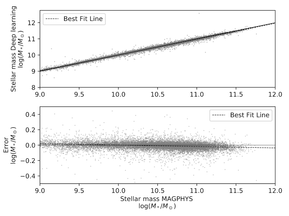
The scatter plot in the upper panel shows the values predicted by the deep learning model compared to the MAGPHYS values, for a specific parameter. The dashed line shows the best linear fit through the scatter plot. The solid line represents the points where the predicted values equal the MAGPHYS model values. The lower panel shows the error in the prediction as a function of the specific parameter.

Scatter plot and error plot for dust luminosity
 Scatter plot and error plot for stellar mass
Scatter plot and error plot for stellar mass
Scatter plot and error plot for star formation rate
The fit for stellar mass and dust luminosity is very close to the 45-degree line with very low scatter. Star formation rate has a little more scatter compared to the former two free parameters. The difference plot highlights this.

It is important to note that the values of these free parameters span three orders of magnitude. The same model is able to predict over this entire range of values as deep learning models are able to capture the non-linear relationships between the input flux values and the output free parameters.

This deep learning technique takes three to 30 minutes to train depending on the free parameter being modelled. Once we have a model, the time taken to predict the free parameters for the test data is negligible. To estimate the three star-formation parameters using the MAGPHYS code for 10,000 galaxies would take ~100,000 minutes (about 10 minutes per galaxy) which amounts to about 2.5 months. Time taken to predict the same number of galaxies using a deep learning model is roughly 30 minutes, with most of this time taken up by training. This represents huge savings in time, with potentially larger savings for samples from future large area imaging surveys. 

Further, this model can be modified to give the confidence level of each prediction. Those galaxies whose free parameters the model predicts with low confidence can be investigated and then rerun with the standard stellar population technique. The outcome of this can then be further investigated and changes incorporated in the deep learning model. Thus, the model can get enriched as it encounters more and more data, which enables it to capture more information and patterns contained in the data.

Future outlook

With new telescopes being built, which will have the ability to capture data at a faster rate, the time savings delivered by this deep learning model can be invaluable. As data is being generated at a velocity much higher than what existing models such as MAGPHYS can process in time, this model can have significant applications in astronomy.

Not just for astronomy, but almost every domain is now gathering as much data as they can. This data needs to be processed faster than the data being generated. Such scenarios in addition to the classification and prediction applications also form good use cases for machine learning algorithms.

This article is an adaptation of a research paper published by Shraddha Surana, Yogesh Wadadekar, Omkar Bait and Hrushikesh Bhosale in the Monthly Notices of the Royal Astronomical Society. You can research entire paper here.

Disclaimer: The statements and opinions expressed in this article are those of the author(s) and do not necessarily reflect the positions of Thoughtworks.

Keep up to date with our latest insights